First Steps in Calculus

Johannes Siedersleben, January 2026

Introduction

“All men are mortal. Socrates is a man, so Socrates is mortal.” Here, we are applying a true statement (“all men are mortal”) to a particular object (“Socrates”), and arriving at the conclusion “Socrates is mortal”, another true statement. Are you impressed? Probably not. Let’s try something better.

“A function is differentiable if the derivative exists.” Applying this definition (a true statement) to the product of two differentiable functions produces the product rule in two lines of straightforward calculations, proving that the product is indeed differentiable (another true statement). Integrating the product rule gives the integration-by-parts rule. Taylor's theorem is proven by applying integration by parts as many times as you like or are allowed to, and this is how the power series in Taylor’s formula originates. What does it mean to “integrate the product rule”? This is another way of saying “apply the main theorem of calculus. To prove the latter, you apply the mean value theorem of integration and that of differentiation, and you prove these by applying the intermediate value theorem which, in turn, is proven by applying the theorem on nested intervals, which you prove by applying the theorem of Bolzano-Weierstrass. And this relies on the fact that \(\mathbb{R}\) is complete: there are no holes in \(\mathbb{R}\), every Cauchy sequence converges.

In the companion paper From Naturals to Reals, we present \(\mathbb{R}\) as the smallest complete field containing the rationals \(\mathbb{Q}\). This paper presents a straight path with no gaps from the starting point (\(\mathbb{R}\) is complete) to two pivotal results:

1. The mean value theorem of integration, which states that differentiation and integration are inverse operations.

2. Taylor's theorem.

These results will, in turn, be the starting point of future papers.

I was led by these rules:

1. No detours, no blind alleys, no embellishments. Every definition, every theorem serves a purpose.

2. No proof when it’s obvious. Example: Proving the linearity of differentiation or integration is a useful exercise, but it is boring and unilluminating. I left it out.

3. No proof when it’s not part of the story. Example: Proving the Lebesgue criterion is hard work and not essential for what follows. I left the proof out, but the criterion is too interesting to be passed over.

4. Full proofs otherwise. The chain of reasoning is complete from the start to the end. This was the point of my opening example.

We restrict ourselves to finite intervals \([a, b]\) for no other reason than to keep the paper short. The backbone of our story is formed by the vector spaces \(\mathcal{R}([a, b])\) of Riemann-integrable functions, and the spaces \(C^n([a, b])\) of \(n\) times continuously differentiable functions. The integral operator \(\int\) shifts functions to the right from \(\mathcal{R}([a, b])\) to \(C^{0}([a, b])\) and further on to \(C^{n}([a, b])\), and the differential operator \(\partial\) shifts them to the left from \(C^n([a, b])\) to \(C^{n-1}([a, b])\), see The Backbone.

Note: I prefer the symbol \(\partial\) for the differential operator over the more frequent \(D\).

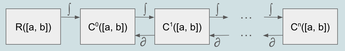
Fig. 2 The Backbone

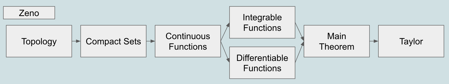
Fig. 3 The Roadmap

Here is the roadmap: After warming up with Zeno’s paradoxes, we study the topology of \(\mathbb{R}\) and compact sets including the Bolzano-Weierstrass theorem, which is indispensable whenever sequences are supposed to converge.

We then turn to continuous functions. On compact sets, they are uniformly continuous and form a vector space closed under the sup-norm. A key result is the intermediate value theorem.

The next two chapters are independent and can be read in any order.

Riemann integrals can be introduced by either Riemann sums or step functions. We show the equivalence of these two approaches. They are equally important; later on, we will use whichever is more appropriate. Riemann-integrable functions also form a vector space closed under the sup-norm. A key result is the mean value theorem of integration, which depends on the intermediate value theorem.

In the chapter on differentiable functions, we prove the well-known differentiation rules. A key result is the mean value theorem of differentiation, which also depends on the intermediate value theorem.

Integration and differentiation are then combined in the mean value theorem of integration. Its proof is a simple application of the mean value theorems of integration and differentiation. The integration rules then follow effortlessly from the differentiation rules and the main theorem. We see that, for the limit of differentiable functions to be differentiable, the derivatives must be uniformly convergent; the vector spaces \(C^{n}([a, b])\) are not closed under the sup-norm.

The apogee of this short paper is Taylor's theorem, which is proven by a simple application of integration by parts.

This material has been published many times, see [Courant, 1955], [Rudin, 1976], [Heuser, 2009], [Forster, 2016], to name but a few prominent examples.

Zeno’s Paradoxes

Calculus is all about infinitesimally small numbers, a subject the Greeks didn’t understand. Zeno’s paradoxes aren’t paradoxes anymore; today, they are easily explained.

Achilles and the Tortoise

Imagine the tortoise and Achilles starting a race with the tortiose \(10\) metres in the lead, and Achilles running ten times as fast as the tortoise.
By the time Achilles has covered \(10\) meters, the tortoise is \(1\) metre in the lead.
By the time Achilles has covered \(11\) meters, the tortoise is \(0.1\) metres in the lead.
By the time Achilles has covered \(11.1\) meters, the tortoise is \(0.01\) metres in the lead.
And so on. Will Achilles ever overtake the tortoise?

Of course, he will after \(11.111\ldots\) metres because

\[\sum_{k=0}^\infty \alpha^k = \frac{1}{1-\alpha}\]

which gives, with \(\alpha = 1/10\):

\[10 + \sum_{k=0}^\infty \frac{1}{10^k} = 10 + \frac{10}{9} = 11.111\ldots\]

Without Zeno, the computation would have been easier: Let \(x(t) = 10t\) be Achilles’ position at time \(t\), and \(y(t) = 10 + t\) that of the tortoise. The equation \(x(t) = y(t)\) has the solution \(t = 10/9 = 1.111 \ldots\).

What seemed paradoxical to Zeno is that the sum of an infinite number of terms could be finite. However, all he did was a mental divison of a finite distance into infinitely many parts, the sum of which is obviously the distance given. Today infinite sums are well understood; there is nothing paradoxical about them.

The Standing Arrow

Imagine an arrow flying along a straight line. At any given moment, the arrow occupies a specific position in space. How can it ever move? The answer is given by the theory of integrals we are going to study in detail. Here is a sketch: Let \(v(t)\) be the speed of the arrow at time \(t\). We divide a given time span \([a, b]\) into tiny, but finitely many subintervals \({[t_k, t_{k+1}]}\). Then, the distance \(d\) traveled in the time interval \([a, b]\) is approximated to any accuracy by the so-called Riemann sum

\[d \approx \sum_{k=0}^n v(t_k) (t_{k+1} - t_k)\]

While the first paradox was that a sum with an infinite number of terms could be finite, this paradox is that the sum of a large number of arbitrarily small terms does not vanish. Assigning meaningful values to such sums is what integration theory is all about.

Topology of \(\mathbb{R}\)

Definition 21 (Topology of \(\mathbb{R}\))

Let \(A \subseteq \mathbb{R}\) and \(a \in A\).

(a) Inner Points, Interior, Open Sets

We call \(a\) an inner point of \(A\), iff

\[\exists \epsilon > 0: U_{\epsilon}(a) \subseteq A\]

The interior of \(A\), denoted be \(A°\), is the set of all interior points of \(A\). We clearly have \(A° \subseteq A\). The set \(A\) is open iff \(A° = A\).

(b) Limit Points, Closure, Closed Sets

We call \(a\) an limit point of \(A\), iff

\[\forall \epsilon > 0: U_{\epsilon}(a)- \{a\} \cap A \neq \emptyset\]

This can expressed as: \(a\) is the limit of a sequence \(\{a_n\}\) of points in \(A\) with \(a_n \neq a\).

The set of limit points of \(A\) is denoted by \(A'\).

The set \(A\) is closed iff its complement \(A^c\) is open.

The closure of \(A\), denoted by \(\bar{A}\), is the smallest closed set containing \(A\)

We clearly have \(A \subseteq \bar{A}\).

Lemma 3 (Limit Points)

Let \(A \subseteq \mathbb{R}\). Then:

\[A' \subseteq \bar{A}\]

Proof. Let \(a \in A' - A\). Then, by definition:

\[\forall \epsilon > 0: U_{\epsilon}(a) \cap A \neq \emptyset\]

Let \(B \supseteq A\) be closed, so \(B^c \subseteq A^c\) is open. Assume that \(a \in B^c\). Then, by definition:

\[\exists \epsilon > 0: U_{\epsilon}(a) \subseteq B^c \subseteq A^c\]

which implies the contradiction \(U_{\epsilon}(a) \cap A = \emptyset\), therefore \(a \in B\) for every closed superset of \(A\), hence \(a \in \bar{A}\).

Theorem 23 (Nested Intervals)

Let \(\{x_n\}\) be a non-decreasing, \(\{y_n\}\) a non-increasing real sequence satisfying:

(44)\[\begin{split}&\forall n \in \mathbb{N}: x_n \le y_n \\ \\ &\lim_{n \to \infty} (y_n - x_n) = 0\end{split}\]

Then \(\{x_n\}\) and \(\{y_n\}\) converge to the same point:

\[\lim_{n \to \infty} x_n = \lim_{n \to \infty} y_n\]

This means that the sequence of intervals \(\{[x_n, y_n]\}\) contracts to one point.

Proof. We show that \(\{x_n\}\) is a Cauchy sequence. For \(m > n\), we have:

\[x_n \le x_m \le y_m \le y_n\]

Subtracting \(x_n\) gives:

\[0 \le x_m - x_n \le y_n - x_n\]

which is what we want because of (44). The sequence \(\{y_n\}\) is a Cauchy sequence by the same argument, and the limits of \(\{x_n\}\) and \(\{y_n\}\) coincide, again because of (44).

Compact Sets

Definition 22 (Compact Sets)

A set \(A \subset \mathbb{R}\) is called compact iff each bounded sequence of elements of A has a convergent subsequence.

Lemma 4 (Completeness, Compactness )

a) Compact sets are complete.

b) Closed subsets of complete sets are complete.

c) Closed subsets of compact sets are compact.

Proof. a) Let \(A \subseteq \mathbb{R}\) be compact and \(\{x_n\}\) a Cauchy-sequence of elements of \(A\). Then, the set \(\{x_n \mid n \in \mathbb{N} \}\) is bounded and has a subsequence that converges to some \(x \in A\). Therefore \(\{x_n\}\), being a Cauchy-sequence, converges itself to \(x\).

b) Let \(A \subseteq \mathbb{R}\) be complete, \(B \subseteq A\) be closed, and \(\{x_n\}\) a Cauchy-sequence of elements of \(B\). Then \(\{x_n\}\) converges because \(A\) is complete, and it converges to some \(x \in B\), because \(B\) is closed.

c) Let \(A \subseteq \mathbb{R}\) be compact, \(B \subseteq A\) be closed, and \(\{x_n\}\) a sequence of elements of \(B\). Then \(\{x_n\}\) has a convergent subsequence because \(A\) is compact, and this subsequence converges to some \(x \in B\), because \(B\) is closed.

Theorem 24 (Supremum, Infimum)

Let \(A \subset \mathbb{R}\) bounded above. Then there is a least upper bound of \(A\), called supremum of \(A\), or \(\sup A\).
Let \(A \subset \mathbb{R}\) bounded below. Then there is a greatest lower bound of \(A\), called infimum of \(A\), or \(\inf A\).

Proof. We prove the assertion for the supremum. Let \(b_0\) be an upper bound of \(A\) and \(a_0 \in A\) any element. We define nested intervals \(\{[a_n, b_n]\}\) as follows:

\[ \begin{align}\begin{aligned}\begin{split}\\ &a_{n+1} = \left\{ \begin{array}{lr} a_n & \text{ if } (a_n + b_n)/2 \notin A \\ (a_n + b_n)/2 & \text{ if } (a_n + b_n)/2 \in A \end{array} \right . \\ \\\end{split}\\\begin{split}&b_{n+1} = \left\{ \begin{array}{lr} (a_n + b_n)/2 & \text{ if } (a_n + b_n)/2 \notin A \\ b_n & \text{ if } (a_n + b_n)/2 \in A \end{array} \right .\end{split}\end{aligned}\end{align} \]

The sequence \(\{[a_n, b_n]\}\) fulfills the prereqisites of Theorem 23. It therefore contracts to some point \(b\) which is an upper bound of \(A\) because all \(b_n\) are. And no upper bound of \(A\) can be smaller than \(b\) because, for any \(\epsilon > 0\), there are \(a_n \in A\) with \(a_n > b - \epsilon\).

Theorem 25 (Bolzano-Weierstrass)

a) Every bounded and monotonous sequence of reals is convergent.

b) Each closed interval \([a, b] \subset \mathbb{R}\) is compact.

Proof. a) Let \(\{x_n\}\) be a non-decreasing bounded sequence with \(s = \sup \{x_n \mid n \in \mathbb{N} \}\). This supremum exists thanks to Theorem 24. We show that \(\{x_n\}\) is a Cauchy-sequence. By the definition:

\[\forall \epsilon > 0 : \exists n(\epsilon) : s - x_{n(\epsilon)} < \epsilon\]

hence, by monotony:

\[\forall \epsilon > 0 : \exists n(\epsilon) :\forall n \ge n(\epsilon) : s - x_{n} < \epsilon\]

The triangular inequality gives us, for \(m,n > n(\epsilon)\)

\[ \left |x_{m} - x_{n} \right | \le \left |x_{m} - s \right | + \left |s - x_{n} \right | < 2\epsilon\]

hence:

\[\forall \epsilon > 0 : \exists n(\epsilon) :\forall n, m \ge n(\epsilon) : \left |x_{m} - x_{n} \right | < 2\epsilon\]

So, \(\{x_n\}\) is a Cauchy sequence and converges to \(s\) by construction.

b) Let \([a, b] \subset \mathbb{R}\) be a closed interval and \(\{x_n\}\) a sequence in \([a, b]\). We are going to show that \(\{x_n\}\) contains a monotounous subsequence that is bounded because everything happens in \([a, b]\).

We call \(m\) a peak, if \(x_n < x_m\) for all \(n > m\). If there are infinitely many peaks \(\{m_k\}\) then \(\{x_{m_k}\}\) is decreasing, and we are done. If not, there is a last peak \(m^*\), and an index \(n_1 > m^*\) that is not a peak. \(n_1\) being not a peak, there must be an index \(n_2 > n_1\) with \(x_{n_2} > x_{n_1}\). And so on. We end up with an increasing sequence \(\{x_{n_k}\}\), which proves the theorem.

Continuous Functions

Definition 23 (Sup Norm)

Let \(f: [a, b] \to \mathbb{R}\) be a bounded function.

The sup norm (or uniform norm) of \(f\) is defined as:

\[\left \lVert f \right \rVert_{\infty} = \sup \{\lvert f(x) \rvert \mid x \in [a, b]\}\]

Remark 8 (Sup Norm)

The sup norm indeed a norm because:

(i) \(f = 0 \Leftrightarrow \left \lVert f \right \rVert_{\infty} = 0\)

(ii) \(\left \lVert \alpha f \right \rVert_{\infty} = \lvert\alpha\rvert \left \lVert f \right \rVert_{\infty}\)

(iii) \(\left \lVert f + g \right \rVert_{\infty} \le \left \lVert f \right \rVert_{\infty} + \left \lVert g \right \rVert_{\infty}\)

The proofs are trivial.

Definition 24 (Convergence of Functions)

Let \(f_n: [a, b] \to \mathbb{R}\) \((n \in \mathbb{N})\) be a sequence of functions, and \(f: [a, b] \to \mathbb{R}\) another function.

(a) We say that \(\lim_{n \to \infty} f_n = f\) pointwise if, for all \(x \in [a, b]\), we have

\[\lim_{n \to \infty} \left | f_n(x) - f(x) \right | = 0\]

(b) We say that \(\lim_{n \to \infty} f_n = f\) uniformly iff

\[\lim_{n \to \infty} {\left \lVert f_n - f \right \rVert_{\infty}} = 0\]

Definition 25 (Continuity)

Let \(f: [a, b] \to \mathbb{R}\) be a function.

(a) \(f\) is continuous at \(x \in [a, b]\) iff

\[\forall \epsilon > 0 : \exists \delta > 0 : \forall h \in [-\delta, \delta ]: \left | f(x + h) - f(x) \right | < \epsilon \]

(b) \(f\) is continuous on \([a, b]\) iff \(f\) is continuous at each \(x \in [a, b]\).

(c) \(f\) is uniformly continuous on \([a, b]\) iff

\[\forall \epsilon > 0 : \exists \delta > 0 : \forall x \in [a, b], h \in [-\delta, \delta]: \left | f(x + h) - f(x) \right | < \epsilon \]

For \(f\) to be uniformly continuous we require that one \(\delta\) do the job for the whole interval \([a, b]\).

Theorem 26 (Continuous Functions on Intervals)

Let \(f: [a, b] \to \mathbb{R}\) be continuous. Then:

(a) The continuous functions on \([a, b]\) form a vector space, written as \(C^0([a, b])\)

(b) The uniform limit of continuous functions is continuous, or: \(C^0([a, b])\) is closed under the sup-Norm.

(c) Continuous function assume their maximum and minimum on \([a, b]\).

(d) Continuous functions are uniformly continuous on \([a, b]\).

Proof. Assertion (a) is obvious. We prove (b) with the triangular inequality. For (c) and (d) we need Bolzano-Weierstrass.

(b) Let \(\{f_n\}\) be a sequence of functions on \([a, b]\) that converges uniformly to \(f\). Let \(\epsilon >0\), \(x \in [a, b]\), \(n \in \mathbb{N}\) such that \(\lVert f_n - f \rVert_{\infty} < \epsilon\) and \(\delta > 0\) such that \( \lvert f_n(x+h) - f_n(x) \rvert < \epsilon\) whenever \(\lvert h \rvert < \delta\). Then:

\[\begin{split}& \lvert f(x+h) - f(x) \rvert \\ & \le \lvert f(x+h) - f_n(x+h) \rvert + \lvert f_n(x+h) - f_n(x) \rvert + \lvert f_n(x) - f(x) \rvert \\ & < 3 \epsilon\end{split}\]

(c) We prove the assertion for the maximum. Let \(M = \sup\{f(x) \mid x \in [a, b] \}\). Then, for each \(n \in \mathbb{N}\), there is a \(x_n \in [a, b]\) such that \(M - f(x_n) < 1/n\). The sequence \(\{x_n\}\) has a subsequence that converges to some \(x \in [a, b]\) because \([a, b]\) is compact, and we have \(f(x) = M\) because \(f\) is continuous at \(x\).

(d) We prove the assertion by contradiction. Assume \(f\) to be not uniformly continuous. Then, for any \(\epsilon > 0\), there exist two sequences \(\{x_n\}, \{y_n\}\) such that

\[\lvert x_n - y_n \rvert < \frac{1}{n}\]

and

\[\lvert f(x_n) - f(y_n) \rvert > \epsilon\]

But \(\{x_n\}\) has a subsequence \(\{x_{n_k}\}\) that converges to some \(x \in [a, b]\), and \(\{y_{n_k}\}\) necessarily converges to the same \(x\), So, \(f\) is not continuous in \(x\), which is a contradiction.

Theorem 27 (Intermediate Value Theorem)

(a) Let \(f: [a, b] \to \mathbb{R}\) be a continuous function with \(f(a) < 0\) and \(f(b) > 0\). Then there exists a \(\xi \in [a, b]\) such that \(f(\xi) = 0\).

(b) Let \(f: [a, b] \to \mathbb{R}\) be a continuous function and \(\mu\) such that

\[\min\{f(x) \mid x \in [a, b]\} \le \mu \le \max\{f(x) \mid x \in [a, b]\}\]

Then there exists a \(\xi \in [a, b]\) such that \(f(\xi) = \mu\).

Proof. (a) We define nested intervals \(\{[a_n, b_n]\}\) as follows:

\[ \begin{align}\begin{aligned}\begin{split}&a_0 = a \\ &b_0 = b \\ \\ &a_{n+1} = \left\{ \begin{array}{lr} a_n & \text{ if } f((a_n + b_n)/2) \ge 0 \\ (a_n + b_n)/2 & \text{ if } f((a_n + b_n)/2) < 0 \end{array} \right . \\ \\\end{split}\\\begin{split}&b_{n+1} = \left\{ \begin{array}{lr} (a_n + b_n)/2 & \text{ if } f((a_n + b_n)/2) \ge 0 \\ b_n & \text{ if } f((a_n + b_n)/2) < 0 \end{array} \right .\end{split}\end{aligned}\end{align} \]

Th sequence \(\{[a_n, b_n]\}\) fulfills the prerequisites of Theorem 23. It therefore contracts to some point \(\xi \in [a, b]\). We observe that, for all \(n\):

\[f(a_n) < 0 \le f(b_n)\]

This implies, because \(f\) is continuous:

\[f(\xi) = 0\]

(b) follows from (a): Choose \(a_0, b_0 \in [a, b]\) such that \(f(a_0) = \min\{f(x) \mid x \in [a, b]\}\) and \(f(b_0) = \max\{f(x) \mid x \in [a, b]\}\). Assume w.l.o.g. that \(a_0 < b_0\) and replace \(f\) with \(f - \mu\).

Riemann-Integrable Functions

There are (at least) two equivalent ways of introducing Riemann integrals: One is based on Riemann sums (or intermediate sums), the other on step functions (or lower and upper sums). While these approaches look very similar, their equivalence, shown in Theorem 28, is not obvious. Step functions are useful when we prove the integrability of certain functions, and Riemann sums are needed for the main theorem of calculus and, later on, for the famous integral theorems of Gauss and Stokes.

Definition 26 (Riemann Integrals by Riemann Sums)

We consider a closed interval \([a, b] \subset \mathbb{R}\) and a function \(f: [a, b] \to \mathbb{R}\).

(a) A partition of \([a, b]\) is a strictly increasing sequence \(X = \left\{x_0, x_1, \dots, x_n\right\}\) with \(a = x_0\), \(b = x_n\). Its granularity is \(\mu(X) = \max \left\{\lvert x_k - x_{k-1} \rvert \mid k=1, \dots, n\right\}\). A sequence \(\xi = \left\{\xi_0, \xi_1, \dots, \xi_{n-1}\right\}\) with \(\xi_k \in [x_{k-1}, x_k)\) is called a set of intermediate points of \(X\).

(b) The Riemann sum of \(f, X, \xi\) is defined as:

\[R(f, X, \xi) = \sum_{k=0}^{n-1} f(\xi_k)(x_{k+1} - x_{k})\]

(c) We say that \(f\) is Riemann-integrable, or R-integrable for short, iff there is a \(A \in \mathbb{R}\) such that:

\[\forall \epsilon > 0: \exists \delta > 0: \left | A - R(f, X, \xi) \right | < \epsilon\]

for all partitions \(X\) with \(\mu(X) < \delta\) and any set \(\xi\) of intermediate points of \(X\).

In this case, we define:

\[\int_a^b f(x) \, dx = A\]

In other words, Riemann sums approximate Riemann integrals to arbitrary precision. We often write:

\[\int_a^b f(x) \, dx \approx \sum_{k=0}^{n-1} f(\xi_k)(x_{k+1} - x_{k})\]

as a short version of the exact definition. This should be read as follows: “For sufficiently fine-grained partitions \(X\), the difference between the left and right sides becomes arbitrarily small for any set \(\xi\) of intermediate points.”

Whenever we prove theorems on Riemann integrals, we are allowed to replace the integrals with Riemann sums of sufficiently small granularity.

Definition 27 (Riemann Integrals by Step Functions)

We consider a closed interval \([a, b] \subset \mathbb{R}\) and a partition \(X\) of \([a, b]\).

(a) A function \(\phi: [a, b] \to \mathbb{R}\) is called a step function iff it is constant on each interval \([x_k, x_{k+1})\) of some partition \(X = \left\{x_0, x_1, \dots, x_n\right\}\) of \([a, b]\). This partition is called \(X_{\phi}\), the associated partition of \(\phi\).

(b) The Riemann sum \(R(\phi, X_{\phi}, \xi)\) of a step function \(\phi\) does not depend on \(\xi\), and we can define:

\[R(\phi) = R(\phi, X_{\phi}, x)= \sum_{k=0}^{n-1} \phi(x_k)(x_{k+1} - x_k)\]

(c) We say that \(f\) is S-integrable, iff

(45)\[\sup_{\phi \le f} R(\phi) = \inf_{\psi \ge f} R(\psi)\]

where \(\phi\) and \(\psi\) range over all step functions on \([a, b]\).

Theorem 28 (Equivalence of R- and S-Integrals)

We consider a closed interval \([a, b] \subset \mathbb{R}\) and a function \(f: [a, b] \to \mathbb{R}\).

Theorem: \(f\) is R-integrable iff it is S-integrable. In this case, we have:

(46)\[\int_a^b f(x) \, dx = \sup_{\phi \le f} R(\phi) = \inf_{\psi \ge f} R(\psi)\]

where \(\phi\) and \(\psi\) range over all step functions on \([a, b]\).

This equivalence allows us to forget the term “S-integrability”.

Proof. Part One: We show that (45) and (46) hold if \(f\) is R-integrable.

Take any \(\epsilon > 0\). Since \(f\) is integrable, there is a partition \(X\) such that:

(47)\[\left | \int_a^b f(x) \, dx - R(f, X, \xi) \right | < \epsilon\]

for any set \(\xi\) of intermediate points of \(X\). We are done if we can produce step functions \(\phi\) and \(\psi\) such that:

(48)\[R(\phi) - \epsilon \le \int_a^b f(x) \, dx \le R(\psi) + \epsilon \]

Here they are:

\[\begin{split}&u_k = \inf \{f(x) \mid x \in [x_{k}, x_{k+1})\} \\ &v_k = \sup \{f(x) \mid x \in [x_{k}, x_{k+1})\} \\ \\ &\phi(x) = u_k \text{ if } x \in [x_{k}, x_{k+1}) \\ &\psi(x) = v_k \text{ if } x \in [x_{k}, x_{k+1}) \\\end{split}\]

The suprema and infima exist because \(f\) is bounded. We conclude:

\[\phi \le f \le \psi \]

from which it follows that:

(49)\[R(\phi) \le R(f, X, \xi) \le R(\psi) \]

for any partition \(X\) and and any set \(\xi\) of intermediate points of \(X\). Combining (49) with (47), we get:

\[R(\phi) - \epsilon \le \int_a^b f(x) \, dx \le R(\psi) + \epsilon\]

for any \(\epsilon > 0\) and this is (48), the inequality we are after.

Part Two: We show that \(f\) is R-integrable if (45) holds.

Take any \(\epsilon > 0\) and choose step functions \(\phi, \psi\) on \([a, b]\) that squeeze \(f\) from below and above:

\[\begin{split}&\phi \le f \le \psi \\ &R(\psi) - R(\phi ) \le \epsilon\end{split}\]

We assume w.l.o.g. that \(\phi\) and \(\psi\) share the same partition \(T = \{t_0, t_1, \ldots, t_m \}\). We are done if we can produce a \(\delta > 0\) such that:

(50)\[R(\phi) - \epsilon \le R(f, X, \xi) \le R(\psi) + \epsilon\]

for any partition \(X\) with \(\mu(X) < \delta\) and any set \(\xi\) of intermediate points of \(X\).

The key idea is to split \([a, b]\) into a “good” set \(U\) and a “bad” set \(V\) and to make \(V\) arbitrarily small.

We are given \(\epsilon\) and \(T\). We choose a partition \(X\) with small \(\delta = \mu(X)\). Each X-interval \([x_k, x_{k+1})\) either fits into one of the T-intervals:

\[[x_k, x_{k+1}) \subseteq [t_j, t_{j+1})\]

or it straddles one of the \(t_j\):

\[x_k \le t_j \le x_{k+1}\]

The latter case occurs at most \(m\) times because there are exactly \(m\) points in \(T\).

We define a step function \(\rho\) by:

\[\rho(x) = f(\xi_k) \text{ for } x \in [x_k, x_{k+1})\]

Note that:

(51)\[R(\rho) = R(f, X, \xi)\]

Let \(U\) be the union of all the intervals in \(X\) that fit into one of the intervals in \(T\), and \(V\) the complement of \(U\).

\[\begin{split}&K = \{k < n \mid \exists j < m: [x_k, x_{k+1}) \subseteq [t_j, t_{j+1}) \} \\ &L = \{k < n \mid k \notin K \} \\ &U = \bigcup_{k \in K} [x_k, x_{k+1}) \\ &V = \bigcup_{k \in L} [x_k, x_{k+1}) \end{split}\]

We have for \(x \in [x_k, x_{k+1}) \subseteq [t_j, t_{j+1})\):

\[\phi(x) = \phi(\xi_k) \le f(\xi_k) = \rho(x) \le \psi(\xi_k) = \psi(x)\]

Therefore, we have on \(U\):

(52)\[\phi(x) \le \rho(x) \le \psi(x)\]

Summing over (52) gives:

(53)\[\sum_{k \in K} \phi(x_k)(x_{k+1} - x_k) \le \sum_{k \in K} \rho(x_k)(x_{k+1} - x_k) \le \sum_{k \in K} \psi(x_k)(x_{k+1} - x_k) \]

The length of \(V\) is bounded by \(m\delta\) because \(V\) contains at most \(m\) intervals, and the length of each interval is less or equal \(\delta\). And, since \(f\) is bounded, there is an \(M \in \mathbb{R}\) such that we have on \(V\):

(54)\[\phi(x) - M \le \rho(x) \le \psi(x) + M\]

Summing over (54) gives:

(55)\[\begin{split}&\sum_{k \in L} \phi(x_k)(x_{k+1} - x_k) - Mm\delta \\ &\le \sum_{k \in L} \rho(x_k)(x_{k+1} - x_k) \\ &\le \sum_{k \in L} \psi(x_k)(x_{k+1} - x_k) + Mm\delta\end{split}\]

The inequalities (53) and (55) are combined to:

\[R(\phi) - Mm\delta \le R(\rho) \le R(\psi) + Mm\delta\]

Remembering (51) and setting \(\delta = \epsilon/Mm\), we arrive at (50), the desired result:

\[R(\phi) - \epsilon \le R(f, X, \xi) \le R(\psi) + \epsilon \]

A famous non-integrable function is the Dirichlet function, which is \(1\) for rational numbers and \(0\) otherwise. It is not integrable because on every interval you’ll find Riemann sums equal to \(0\), and others equal to \(1\).

Definition 28 (Riemann Primitives)

Let \(f \in \mathcal{R}([a,b])\). The function \(F\) defined by

\[F(x) = \int_a^x f(y) \, dy \]

is called the Riemann-primitive (or primitive) of \(f\), on the understanding that

\[F(a) = \int_a^a f(x) \, dx = 0\]

The notation

\[F = \int f(y) \, dy\]

is used if the lower bound \(a\) is unimportant or not specified. Two primitives of an integrable function \(f\) differ only by a constant (see additivity).

Theorem 29 (Properties of Riemann Integrals)

We state some obvious but important properties of Riemann integrals.

(a) Boundedness

R-integrable functions are bounded on closed intervals (because Riemann sums are).

(b) Monotony

\[f \le g \Rightarrow \int_a^b f(x) \, dx \le \int _a^b g(x) \, dx\]

holds for any two functions \(f,g \in \mathcal{R}([a,b])\).

(c) Triangular Inequality

If \(f\) is integrable, then so is \(|f|\), and it holds that:

\[\left | \int_a^b f(y) \, dy \right | \le \int_a^b \left | f(y) \right | \, dy \]

(d) Additivity

Let \(f\) be integrable, and \(c \in [a, b]\). Then it holds that:

\[\int_a^b f(x) \, dx = \int_a^c f(x) \, dx + \int_c^b f(x) \, dx\]

(e) Linearity

If \(f, g\) are integrable, then so is \(f + \alpha g\) (\(\alpha \in \mathbb{R}\)), and it holds that:

\[\int_a^b f(x) + \alpha g(x) \, dx = \int_a^b f(x) \, dx + \alpha \int_a^b g(x) \, dx\]

(f) The R-integrable functions over \([a, b]\) form a vector space, written as \(\mathcal{R}([a, b])\).

(g) The primitive of an R-integrable function is continuous. The mapping

\[\begin{split}\int : \left\{ \begin{array}{lr} \mathcal{R}([a, b]) \to C^0([a, b]) \\ f \mapsto \int_a^x f(y) \, dy \end{array} \right .\end{split}\]

is a linear operator, called the integration operator.

The mapping

\[\begin{split}\int : \left\{ \begin{array}{lr} \mathcal{R}([a, b]) \to \mathbb{R} \\ f \mapsto \int_a^b f(y) \, dy \end{array} \right .\end{split}\]

is a linear mapping, called the integration functional.

Proof. We only prove (g).

Let \(f: [a, b] \to \mathbb{R}\) be integrable, and \(F\) a primitive of \(f\). Then, \(f\) is bounded by some \(M \in \mathbb{R}\), and by the triangular inequality (c), we have for \(x \in [a, b]\) and arbitrarily small \(h\):

\[\left | F(x+h) - F(x) \right | = \left | \int_x^{x+h} f(y) \, dy \right | \le \int_x^{x+h} \left | f(y) \right | \, dy \le h M\]

which proves the continuity of \(F\) at \(x\).

We now introduce some criteria of Riemann integrability. The proofs use step functions rather than Riemann sums.

Theorem 30 (Riemann-Integrable Functions)

All functions are defined on a closed interval \([a, b]\).

(a) Step functions are R-integrable and, for any step function \(\phi\) we have:

\[R(\phi) = \int_a^b \phi(x) \, dx\]

(b) Monotonous functions are R-integrable.

(c) Continuous functions are R-integrable.

(d) Let \(f\) be bounded and continuous except on a set \(D\) with a finite number of limit points. Then \(f\) is R-integrable.

Proof. (a) This follows from Theorem 28. We clearly have:

\[\sup_{\varphi \le \phi} R(\varphi) = R(\phi) = \inf_{\psi \ge \phi} R(\psi)\]

The proofs of (b), (c), (d) are very similar. \(f\) can always be squeezed between two suitable step functions \(\phi, \psi\). Here they are:

Take any \(\epsilon > 0\), let \(X\) be a partition, and \(\delta = \mu(X)\). We set for \(k = 0, \ldots, n-1\):

\[\begin{split}& \phi(x) = \inf \{f(x) \mid x \in [x_k, x_{k+1}) \} \\ & \psi(x) = \sup \{f(x) \mid x \in [x_k, x_{k+1}) \}\end{split}\]

The suprema and infima exist because \(f\) is bounded. For (a), (b), and (c), we have to show that:

\[R(\psi) - R(\phi) < \epsilon\]

if \(\mu(X)\) is sufficiently small.

(b) Let \(f\) be non-decreasing. We get:

(56)\[\begin{split}&R(\psi) - R(\phi) = \sum_{k=0}^{n-1} (f(x_{k+1}) - f(x_{k})) (x_{k+1} - x_k) \\ &\le \delta \sum_{k=0}^{n-1} (f(x_{k+1}) - f(x_{k})) \\ &= \delta (f(b) - f(a)) < \epsilon\end{split}\]

if \(\delta < \epsilon /(f(b) - f(a))\).

(c) Let \(f\) be continuous. Then it is uniformly continuous on \([a, b]\) and there is a \(\delta > 0\) such that, for all \(k\), \(\psi(x_k) - \phi(x_{k}) < \epsilon\) if \(\mu(X) < \delta\). We get:

(57)\[\begin{split}&R(\psi) - R(\phi) = \sum_{k=0}^{n-1} (\psi(x_{k}) - \phi(x_{k})) (x_{k+1} - x_k) \\ &< \epsilon \sum_{k=0}^{n-1} (x_{k+1} - x_k) \\ &= \epsilon (b - a)\end{split}\]

In (56) and (57) we encounter collapsing sums, which are a recurrent pattern in the theory of integrals.

(d) Let \(f\) be bounded, continuous and \(D\) the set of points where \(f\) is discontinous. We assume that \(D\) has only one limit point \(d^*\). If there is more than one, simply divide \([a, b]\) into as many subintervals with one limit point in each.

We split the interval \([a, b]\) into a “good” set \(U\) and a “bad” set \(V\), as we did in the proof of Theorem 28.

\[\begin{split}&K = \{k < n \mid D \cap [x_k, x_{k+1}) = \emptyset \} \\ &L = \{k < n \mid k \notin K \} \\ &U = \bigcup_{k \in K} [x_k, x_{k+1}) \\ &V = \bigcup_{k \in L} [x_k, x_{k+1})\end{split}\]

Since \(f\) is uniformly continuous on \(U\), there is a \(\delta > 0\) such that, for all \(k \in K\), \(\psi(x_k) - \phi(x_{k}) < \epsilon\) if \(\mu(X) < \delta\). We have on \(U\):

(58)\[\sum_{k\in K} (\psi(x_{k}) - \phi(x_{k})) (x_{k+1} - x_k) \le \epsilon (b-a)\]

Since \(|d - d^*| < \delta\) for all but finitely many \(d \in D\), all but finitely many elements of \(D\) are assembled in just one interval \([x_k, x_{k+1})\), however small \(\delta\) is. Therefore the number of elements of \(L\), say \(m\), is finite. And \(|f|\) is bounded by some real number \(M\). We have on \(V\):

(59)\[\sum_{k\in L} (\psi(x_{k}) - \phi(x_{k})) (x_{k+1} - x_k) \le \delta m M\]

Adding (58) and (59) gives us:

\[\begin{split}\sum_{k=0}^{n-1} (\psi(x_{k}) - \phi(x_{k})) (x_{k+1} - x_k) \le \epsilon (b-a) + \delta m M \\\end{split}\]

or:

\[R(\psi) - R(\phi) \le \epsilon (b-a) + \delta m M\]

Setting \(\delta = \epsilon/mM\) gives us what we want.

Remark 9 (Lebesgue Criterion)

The story of Theorem 30 doesn’t end here. The ultimate result is the Lebesgue Criterion, the proof of which is too lengthy for this short introduction. To state it, we first need a definition:

A set \(A \subset \mathbb{R}\) has measure zero, iff, for any \(\epsilon > 0\) there is a covering \(C\) of \(A\) with \(|C| < \epsilon\).

Here is the Lebesgue Criterion:

Bounded functions are R-integrable iff their set of discontinuities has measure zero.

Theorem 31 (Uniform Limit of Riemann Integrable Functions)

The uniform limit of R-integrable functions is R-integrable, or, equivalently: \(\mathcal{R}([a, b])\) is closed under the sup norm. We can swap limit and integral:

(60)\[\lim_{n \to \infty} \int_a^b f_n(x) \, dx = \int _a^b\lim_{n \to \infty} f_n(x) \, dx\]

Proof. Let \(\{f_n\}\) be a sequence of R-integrable functions on \([a, b]\) that converges uniformly to \(f\). Let \(\epsilon >0\) and \(n_0\) be such that, for \(n \ge n_0\):

\[\left \lVert f_n - f \right \rVert_{\infty} < \epsilon \]

which implies for any partition \(X\) and any set \(\xi\) of intermediate points:

\[\left | R(f_n, X, \xi) - R(f, X, \xi) \right | < \epsilon (b - a)\]

Let \(\phi_n, \psi_n\) be step functions such that

\[\begin{split}&\phi_n \le f_n \le \psi_n \\ &R(\psi) - R(\phi) < \epsilon\end{split}\]

which implies:

\[R(\phi) - \epsilon (b-a) \le R(f, X, \xi) \le R(\psi) + \epsilon (b-a)\]

whenever \(X\) is as least as fine grained as \(X_{\phi}\) and \(X_{\psi}\). This proves that \(f\) is integrable. Equation (60) follows from:

\[\left | \int_a^b f_n(x) \, dx - \int_a^b f(x) \, dx \right | \le \int_a^b \left | f_n(x) - f(x) \right | \, dx \le (b - a) \left \lVert f_n - f \right \rVert_{\infty}\]

Theorem 32 (Mean Value Theorem of Integration)

Let \(f,\phi : [a, b] \to \mathbb{R}\) be continuous functions with \(\phi \ge 0\).

Then there exists a \(\xi \in [a, b]\) such that:

\[\int _a^b f(x) \phi(x) \, dx = f(\xi) \int _a^b \phi(x) \, dx\]

With \(\phi = 1\) we get:

\[\int_a^b f(x) \, dx= f(\xi) (b-a)\]

Proof. From Theorem 27 we know that there exists a \(\xi \in [a, b]\) such that \(f(\xi) = \mu\). And, \(f\) being bounded on \([a,b]\), we have, for \(x \in [a,b]\):

\[m \le f(x) \le M \]

The rest is straightforward: multiply by \(\phi(x)\) and integrate:

\[ \begin{align}\begin{aligned}& m \phi(x) \le f(x) \phi(x) \le M \phi(x)\\& \Rightarrow m \int_a^b \phi(x) \, dx \le \int_a^b f(x) \phi(x) \, dx \le M \int_a^b \phi(x) \, dx \\& \Rightarrow \int _a^b f(x) \phi(x) \, dx = \mu \int_a^b \phi(x) \, dx = f(\xi) \int_a^b \phi(x) \, dx \end{aligned}\end{align} \]

Differentiable Functions

Definition 29 (Derivatives)

We consider a closed interval \([a, b] \subset \mathbb{R}\) and a function \(f:[a, b] \rightarrow \mathbb{R}\).

(a) We say that \(f\) is differentiable at \(x \in [a, b]\) if the limit

(61)\[\lim_{h \to 0} \frac{1}{h}(f(x+h)-f(x)) = f'(x)\]

exists. \(f'(x)\) is called the derivative of \(f\) at \(x\). We often use the notation:

(62)\[\frac{df}{dx} = f'(x)\]

The statement (61) is equivalent to

(63)\[f(x+h) = f(x) + f'(x) \, h + o(h)\]

which means that the term \(f'(x) \, h\) is a linear approximation of \(f\) at \(x\). The derivative is fully determined by equation (63). From

(64)\[f(x+h) = f(x) + y \, h + o(h)\]

for some value \(y\) we can conclude that \(y = f'(x)\).

(c) We say that \(f\) is continuously differentiable at \(x \in [a, b]\) if it is differentiable at \(x\) and its derivative \(f'\) is continuous at \(x\).

(b) We say that \(f\) is differentiable on \([a, b]\) if it is differentiable for all \(x \in [a, b]\). \(f'\) is called the derivative of \(f\) on \([a, b]\).

(c) We say that \(f\) is continuously differentiable on \([a, b]\) if it is differentiable on \([a, b]\) and its derivative is continuous on \([a, b]\).

(d) Higher order derivatives are analogously defined and denoted by \(f', f'', f^{(3)}, \ldots, f^{(n)}\). A function is said to be \(n\) times continuously differentiable if \(f^{(n)}\) is continuous on \([a, b]\).

Theorem 33 (Properties of Derivatives)

(a) The continuously differentiable functions over \([a, b]\) form a vector space, written as \(C^1 ([a, b])\). Likewise, the \(n\) times continuously differentiable functions over \([a, b]\) form a vector space, written as \(C^n ([a, b])\).

(b) The mapping

\[\begin{split}\partial : \left \{ \begin{array}{lr} C^1 ([a, b]) \to C^0([a, b]) \\ f \mapsto f' \end{array} \right .\end{split}\]

is a linear mapping, called the differential operator.

Likewise, the mapping

\[\begin{split}\partial^2 : \left \{ \begin{array}{lr} C^2 ([a, b]) \to C^0([a, b]) \\ f \mapsto f'' \end{array} \right .\end{split}\]

is again a linear mapping, called the differential operator of second order. Higher order differential operators \(\partial^n\) are analogously defined.

Proof. omitted

Theorem 34 (Differentiation Rules)

(a) Chain Rule

Let \(f \in C^1([a,b])\) and \(g \in C^1([\min(f), \max(f)])\). Then:

\[\begin{split}&(f \circ g)'(x) = (f' \circ g)(x) \, g'(x) \\ \\ &(f \circ g)' = (f' \circ g) \, g'\end{split}\]

(b) Quotient Rule

Let \(f, g \in C^1([a,b])\), and \(f'(x) \ne 0\) on \([a, b]\). Then:

\[{f^{-1}}'(f(x)) = \frac{1}{f'(x)}\]

or, with \(y = f(x)\):

\[{f^{-1}}'(y) = \frac{1}{f'(f^{-1}(y)}\]

This is often abbreviated to

\[{f^{-1}}' = \frac{1}{f'}\]

but you have to keep track of \(x\) and \(y\). Using the quotient notation, we can write:

\[\begin{split}&\frac{df^{-1}}{dy}(f(x)) = \left ( \frac{df}{dx} \right )^{-1}(x) \\ \\ &\frac{df^{-1}}{dy}(y) = \left ( \frac{df}{dx} \right )^{-1}(f^{-1}(y)) \end{split}\]

(c) Product Rule

Let \(f, g \in C^1([a,b])\). Then:

\[f'g' = f'g + fg'\]

Proof. (a) Let \(f, g\) be as above. We prove the assertion using the little-o-notation. We know that \(g\) is differentiable at \(x\), and \(f\) at \(g(x)\).

\[\begin{split}(f \circ g)(x + h) &= f(g(x + h)) \\ \\ &= f(g(x) + g'(x)h + o(h)) \\ \\ &= f(g(x)) + f'(g(x))(g'(x)h + o(h)) + o(g'(x)h + o(h)) \\ \\ &= f(g(x)) + f'(g(x))g'(x)h + f'(g(x))o(h) + o(g'(x)h + o(h))\end{split}\]

Observing that:

\[f'(g(x))o(h) + o(g'(x)h + o(h)) = o(h) + o(h) + o(h) = o(h)\]

we get:

\[(f \circ g)(x + h) = f(g(x)) + f'(g(x))g'(x)h + o(h)\]

which is what we want.

(b) From

\[(f^{-1} \circ f)'(x) = {f^{-1}}'(f(x))f'(x) = 1\]

we conclude:

\[{f^{-1}}'(f(x)) = \frac{1}{f'(x)}\]

(c) Same procedure: \(f\) and \(g\) are differentiable, so:

\[\begin{split}f(x+h)g(x+h) &= (f(x) + f'(x)h + o(h))(g(x) + g'(x)h + o(h)) \\ \\ &= f(x)g(x) + (f'(x)g(x) + f(x)g'(x))h + o(h)\end{split}\]

which is the desired result.

Theorem 35 (Mean Value Theorem of Differentiation)

(a) Minimum, Maximum

Let \(f: [a,b] \to \mathbb{R}\) be differentiable at \(x \in (a,b)\). If \(f\) has a local minimum or maximum in \(x\) then \(f'(x) = 0\).

(b) Rolle’s Theorem

Let \(f: [a,b] \to \mathbb{R}\) be continous and differentiable on \((a,b)\). If \(f(a) = f(b)\) then there is a \(\xi \in (a,b)\) with \(f'(\xi) = 0\).

(c) Mean Value Theorem of Differentiation

Let \(f: [a,b] \to \mathbb{R}\) be continous and differentiable on \((a,b)\) Then there is a \(\xi \in (a,b)\) with:

\[f'(\xi) = \frac{f(b) - f(a)}{b - a}\]

Proof. (a) Let \(x\) be a local maximum. Then, for smalll \(h\):

\[f(x+h) - f(x) \le 0\]

This gives for \(h>0\)

\[\frac{1}{h}(f(x+h) - f(x)) \le 0\]

and for \(h<0\)

\[\frac{1}{h}(f(x+h) - f(x)) \ge 0\]

which implies:

\[\lim_{h \to 0}\frac{1}{h}(f(x+h) - f(x)) = 0\]

(b) \(f\) is either constant or it assumes its minimum and its maximum at some \(\xi \in (a, b)\). We know from (a) that \(f'(\xi) = 0\).

(c) We apply (b) to the function \(g\) defined by

\[g(x) = f(x) - \frac{f(b)- f(a)}{b - a}(x - a)\]

We have \(g(a) = g(b) = f(a)\), and the derivative is:

\[g'(x) = f'(x) - \frac{f(b)- f(a)}{b - a}\]

Through (b) we know that there is a \(\xi \in (a, b)\) with \(g'(x) = 0\). This is the assertion.

Main Theorem of Calculus

Theorem 36 (Main Theorem of Calculus)

Let \(f \in \mathcal{R}([a,b])\) and \(F\) be a primitive of \(f\), defined by

\[F(x) = \int_a^x f(y) \, dy, \quad F = \int f \]

Then:

(a) If \(f\) is continuous on \([a, b]\), then \(F\) is differentiable on \([a, b]\), and it holds that

\[F' = f, \quad \partial \int f = f\]

(b) If \(f\) is differentiable on \([a, b]\), then

\[\int_a^b f'(y) \, dy = f(b) - f(a), \quad \int \partial f = f\]

(c) The linear operators \(\int\) and \(\partial\)

\[\begin{split}\int : \left\{ \begin{array}{lr} C^0([a, b] \to C^1([a, b] \\ f \mapsto F \end{array} \right . \\ \\ \partial : \left\{ \begin{array}{lr} C^1([a, b] \to C^0([a, b] \\ F \mapsto f \end{array} \right .\end{split}\]

are inverse to each other:

\[\int \partial F = F, \quad \partial \int f = f\]

Proof. (a) The proof relies on the mean value theorem of integration. We prove in fact a slightly stronger assertion:

If \(f\) is continuous on a neighbourhood of \(x \in [a, b]\), then \(F'(x) = f(x)\).

Let \(x\) be such a point. Then, for any \(h > 0\) we have:

\[\frac{1}{h}(F(x+h) - F(x)) = \int_x^{x+h} f(y) \, dy = \frac{1}{h} h f(\xi) = f(\xi)\]

for some \(\xi \in [x,x+h]\), and \(f(\xi) \to f(x)\) as \(h \to 0\) since \(f\) is continuous near \(x\).

(b) The proof relies on the mean value theorem of differentiation.

If \(f\) is differentiable, then it is integrable. Let \(\{x_k\}\)be a partition of \([a, b]\), and \(\{\xi_k\}\) a set of intermediate points such that:

\[f'(\xi_k) = \frac{f(x_{k+1}) - f(x_k)}{x_{k+1} - x_k}\]

and we get:

(65)\[\begin{split}\int_a^b f'(y) \, dy &\approx \sum_{k=0}^{n-1}f'(\xi_k)(x_{k+1} - x_k) \\ &= \sum_{k=0}^{n-1}\frac{f(x_{k+1} - f(x_k)}{x_{k+1} - x_k}(x_{k+1} - x_k) \\ &= \sum_{k=0}^{n-1}f(x_{k+1}) - f(x_k) \\ &= f(b) - f(a)\end{split}\]

The final reasoning is standard: We choose partitions \(\{x_k\}\) with arbitrarily small granularity. The approximation in (65) is thus driven to equality. The last equation in (65) is again the collapsing sum pattern.

Theorem 37 (Integration Rules)

Let \(f, g \in C^1([a,b])\)

(a) Integration by Parts

Let \(f, g \in C^1([a,b])\). Then

(66)\[\int^b_a f(x) \, g'(x) \, dx = f \, g \vert^b_a - \int^b_a f'(x) g(x) \, dx\]

(b) Substitution Rule

Let \(f \in C^1([a,b])\) and \(g \in C^1([g^{-1}(a), g^{-1}(b)])\) with \(g' \neq 0\). Then

(67)\[\int_a^b f(g(x))\,g'(x) \, dx = \int_{g(a)}^{g(b)} f(y) \, dy \]

and equivalently with \(u = g(a), v = g(b)\):

(68)\[\int_u^v f(y) \, dy = \int^{g^{-1}(v)}_{g^{-1}(u)} f(g(x))\,g'(x) \, dx\]

Proof. (a) We know from Theorem 34 that:

\[(fg)' = f'g + fg'\]

and with Theorem 36 we conclude:

\[f \, g \vert^b_a = \int_a^b (fg)'(x) \, dx = \int_a^b f'(x)g(x) \, dx + \int_a^b f(x)g'(x) \, dx\]

(b) We know from Theorem 34 that:

\[(f\circ g)'(x) = f'(g(x))g'(x)\]

and with Theorem 36 we conclude:

\[\begin{split}&f \circ g \vert_a^b = \int_{a}^{b} (f \circ g)'(x) \, dx = \int_a^b f'(g(x))g'(x) \, dx \\ &= f(g(a)) - f(g(b)) = \int_{g(a)}^{g(b)} f'(y) \, dy \end{split}\]

Remark 10 (dx Calculus)

The substitution rules (67) and (68) can be memorized as follows:

(69)\[\begin{split}&y = g(x) \\ & \Rightarrow \frac{dy}{dx} = \frac{dg}{dx} = g'(x) \\ & \Rightarrow dy = g'(x) \, dy\end{split}\]

You still have to keep track of the integration bounds.

Theorem 38 (Legendre Substitution)

Let \(f \in C^1([0,x_0])\) with \(f(0) = 0\) and \(f' \neq 0\). Then the Legendre equation holds:

(70)\[\int_0^{x_0} f(x) \, dx + \int_0^{y_0} f^{-1}(y) \, dy = x_0 y_0\]

Proof. We apply equation (68) and integrate by parts:

\[\begin{split}\int_0^{y_0} f^{-1}(y) \, dy &=\int_0^{f^{-1}(y_0)} x f'(x) \, dx \\ &= x f(x) \vert_0^{x_0} - \int_0^{x_0} f(x) dx \\ &=x_0 y_0 - \int_0^{x_0} f(x) dx\end{split}\]

Theorem 39 (Limit of Differentiable Functions)

Let \(\{f_n\}\) converge pointwise to some function \(f\), with \(f_n \in C^1([a,b])\).
Let \(\{f'_n\}\) converge uniformly to some function \(g\). Then \(f\) is differentiable, and \(g = f'\), or:

\[\lim_{n \to \infty} \partial f_n = \partial \lim_{n \to \infty} f_n\]

where the limit is uniform.

Proof. From the main theorem of calculus (a) we get, since all \(f'_n\) are continuous:

\[f_n(x) = f_n(a) + \int_a^x f'_n(y) \, dy\]

From Theorem 31 we get, since the convergence of \(\{f'_n\}\) is uniform::

\[f(x) = \lim_{n \to \infty} f_n(x) = \lim_{n \to \infty} \left ( f_n(a) + \int_a^x f'_n(y) \, dy \right )= f(a) + \int_a^x g(y) \, dy\]

Therefore, again by the main theorem of calculus (a), \(f\) is differentiable and \(f' = g\).

Remark 11 (Counterexample)

The uniform limit of continuously differentiable functions is emphatically not always differentiable. A simple example is:

\[f_n(x) = \sqrt{x^2 + \frac{1}{n}}\]

The uniform limit is the absolute value function that features a corner at \(0\).

\[\lim_{n \to \infty} f_n(x) = |x|\]

Taylor’s Theorem

Derivatives are about local changes: How does a function \(f\) behave in a neighbourhood of some point \(x\)? The Taylor series allows us to express \(f(x+h)\) in terms of the higher derivatives of \(f\) with arbitrary precision. It comes in three varieties that differ in the remainder term.

Theorem 40 (Taylor’s Theorem)

Let \([a, b]\) be a finite interval \(f \in C^{n+1}([a, b])\), \(x \in (a, b)\) and \(h\) so small that \(x+h \in [a, b]\). Then:

(a)

(71)\[f(x+h)=\sum _{k=0}^n \frac{f^{(k)}(x)}{k!}(h)^k + \frac{1}{n!}\int _x^{x+h} (x+h-t)^n f^{(n+1)}(t) \, dt\]

(b) There exists a \(\xi \in [x-h,x+h]\) such that:

(72)\[f(x+h)=\sum _{k=0}^n \frac{f^{(k)}(x)}{k!}h^k + \frac{f^{(n+1)}(\xi)}{(n+1)!}h^{n+1}\]

(c)

(73)\[f(x+h)=\sum _{k=0}^n \frac{f^{(k)}(x)}{k!}h^k + o(h^n)\]

Proof. (a) The proof is by induction, using the main theorem of integration and integration by parts. We set \(u = x+h\).

\[\begin{split}f(u) - f(x) &= \int _x^u f'(t)dt = - \int _x^u\frac{d(u-t)}{dt}f'(t)dt \\ & = -(u-t)f'(t) \lvert_x^u + \int _x^u(u-t)f''(t)dt \\ & = (u-x)f'(x) + \int _x^u(u-t)f''(t)dt = \text{ ... } \\ & =\sum _{k=1}^n \frac{f^{(k)}(x)}{k!}(u-x)^k + \frac{1}{n!}\int _x^u (u-t)^n f^{(n+1)}(t)dt\end{split}\]

We obtain equation (71) by replacing \(u\) with \(h = u-x\).

(b) Using the mean value theorem of integration, we find a \(\xi \in [x-h, x+h]\) such that

\[\frac{1}{n!}\int _x^u(u-t)^nf^{(n+1)}(t)dt = \frac{f^{(n+1)}(\xi)}{n!}\int_x^u (u-t)^n dt = \frac{f^{(n+1)}(\xi)}{(n+1)!}(u-x)^{n+1}\]

We obtain equation (72) again by replacing \(u\) with \(h = u-x\).

(c) This follows from (b), because:

\[\frac{f^{(n+1)}(\xi)}{(n+1)!}h^{n+1} = o(h^n)\]

Little o, Big O

Little o means: \(f\) tends to \(0\) faster than \(g\), or, equivalently, \(f/g\) tends to \(0\):

\[\begin{split}&f = o(g) \Leftrightarrow \lim\frac{f(x)}{g(x)} = 0 \\ \\ &f = o(1) \Leftrightarrow \lim f(x) = 0 \\ \\ &f = o(x^n) \Leftrightarrow \lim \frac{f(x)}{x^n} = 0\end{split}\]

Big O means: \(f\) grows not faster than \(g\), or, equivalently, \(f/g\) is bounded above:

\[\begin{split}&f = O(g) \Leftrightarrow \frac{f(x)}{g(x)} \le C \\ \\ &f = O(1) \Leftrightarrow f(x)\le C \\ \\ &f = O(x^n) \Leftrightarrow f(x)\le C x^n\end{split}\]